SingleWave

class fridom.nonhydro.initial_conditions.single_wave.SingleWave(mset: ModelSettings, k: tuple[int], s: int = 1, phase: float = 0, use_discrete: bool = True)

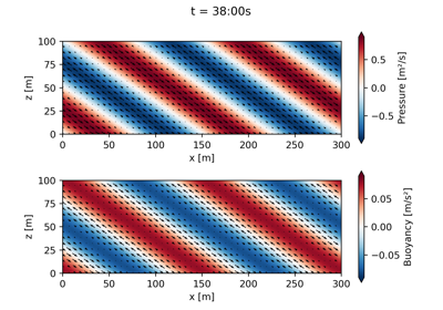
Bases: State

An initial condition that consist of a single wave with a given wavenumber and a given mode.

Description

Creates a polarized wave from the eigenvectors of the linearized equations of motion. The wave is initizalized in spectral space as:

\[z(\boldsymbol{k}) = \boldsymbol{q}_s(\boldsymbol{k}) \delta_{\boldsymbol{k}, \boldsymbol{k}_0} \exp(i\phi)\]

where \(\boldsymbol{q}_s\) is the eigenvector of the mode s (see fridom.nonhydro.grid.cartesian.eigenvectors), and \(\delta_{\boldsymbol{k}, \boldsymbol{k}_0}\) is the Kronecker delta function:

\[\begin{split}\delta_{\boldsymbol{k}, \boldsymbol{k}_0} = \begin{cases} 1 & \text{if } \boldsymbol{k} = 2\pi\boldsymbol{k}_0/\boldsymbol{L} \\ 0 & \text{otherwise} \end{cases}\end{split}\]

with \(\boldsymbol{L}\) the domain size in the x, y, and z directions and \(\boldsymbol{k}_0\) the wavenumber that is passed as an argument. The phase \(\phi\) is also passed as an argument. Finally, the state is fourier transformed to physical space and normalized so that its L2 norm is equal to 1.

Parameters

msetModelSettings

The model settings.

ktuple[int]

The wavenumber in the x, y, and z directions. A wavenumber of one means that the wave has a wavelength equal to the domain size in that direction.

sint

The mode (0, 1, -1) 0 => geostrophic mode 1 => positive inertia-gravity mode -1 => negative inertia-gravity mode

phasefloat

The phase of the wave. (default: 0)

use_discretebool (default: True)

Whether to use the discrete eigenvectors or the analytical ones.

__init__(mset: ModelSettings, k: tuple[int], s: int = 1, phase: float = 0, use_discrete: bool = True) → None

Methods

__init__(mset, k[, s, phase, use_discrete])
dot(other)	Calculate the dot product of the state with another state.
fft([padding])	Calculate the Fourier transform of the state.
from_netcdf(mset, path)	Read the state from a NetCDF file.
has_nan()	Check if the state contains NaN values.
ifft([padding])	Calculate the inverse Fourier transform of the state.
norm_l2()	Calculate the L2 norm of the state.
norm_of_diff(other)	The norm of the difference between two states.
project(p_vec, q_vec)	Project the state on a (spectral) vector.
sync()	Synchronize the state.
to_netcdf(path)	Write the state to a NetCDF file.

Attributes

arr_dict	Return the dictionary of arrays (not FieldVariables).
b	Buoyancy
cfl	The CFL number.
ekin	The kinetic energy
epot	The potential energy
etot	The total energy
field_list	Return the list of fields.
grid	Return the grid of the model.
linear_pot_vort	Linearized potential vorticity
local_Ro	Local Rossby number
pot_vort	Scaled potential vorticity field.
rel_vort	The relative vorticity
rel_vort_x	X-component of the relative vorticity
rel_vort_y	Y-component of the relative vorticity
rel_vort_z	Z-component of the relative vorticity (Horizontal Vorticity)
u	Velocity in the x-direction.
v	Velocity in the y-direction.
w	Velocity in the z-direction.
xr	State as xarray dataset
xrs	State of sliced domain as xarray dataset

Examples using fridom.nonhydro.initial_conditions.SingleWave

Single Internal Wave

Single Internal Wave