Field Variables and Plotting

Field Variables and Plotting#

Note

In this tutorial, we use the xarray library. Ensure that you install it before running the code snippets.

The FieldVariable class is the fundamental class for all fields used in FRIDOM. Essentially, a field variable is a wrapper around multidimensional arrays that can be stored in various backends, such as numpy, cupy, or jax.numpy.

In addition to the array itself, a field variable stores a range of metadata, including the field’s name, units, coordinate information, and dimensions. If you’re familiar with xarray, you’ll notice that the field variable class is very similar to DataArray in xarray. In fact, later in this tutorial, we will see how field variables can be easily converted to xarray DataArrays. This is particularly useful if you want to leverage the extensive plotting capabilities of xarray.

In this tutorial, you will learn how to create field variables, manipulate them, plot them, and explore a variety of useful functions to work with them effectively.

Creating Field Variables#

To create a field variable, you need to provide the ModelSettings object and the name of the field. Additionally, a range of optional arguments can be specified, such as the field’s unit and a longer, more descriptive name. For a full list of possible arguments that can be passed to the field variable class, refer to the API documentation.

In the following example, we create a field variable for temperature:

Creating a field variable#

import fridom.shallowwater as sw

grid = sw.grid.cartesian.Grid(N=(256,256), L=(1,1), periodic_bounds=(True, True))
mset = sw.ModelSettings(grid=grid)
mset.setup()

temperature = sw.FieldVariable(mset, name="temp", units="K", long_name="Temperature")

By default, a field variable is initialized with zeros. Let’s now look at how we can access and manipulate the data within field variables.

Manipulating Field Variables#

Field variables can primarily be manipulated in three ways: through arithmetic operations, built-in methods of the field variable class, and numpy functions.

Arithmetic Operations#

Let’s start with arithmetic operations between field variables and scalars:

Arithmetic operations with scalars#

import fridom.shallowwater as sw

grid = sw.grid.cartesian.Grid(N=(256,256), L=(1,1), periodic_bounds=(True, True))
mset = sw.ModelSettings(grid=grid)
mset.setup()

# Create a field variable
u = sw.FieldVariable(mset, name="u")

# We can access the data of the field variable using the .arr attribute
print(u.arr)  # 0 everywhere

# Adding a scalar to the field variable
u += 3.14  # or alternatively: u = u + 3.14

print(u.arr)  # 3.14 everywhere

In addition to addition, subtraction (-), multiplication (*), division (/), and exponentiation (**) with scalars are also supported.

We can also perform these arithmetic operations between two field variables. When performing arithmetic operations between two field variables, the attributes of the first field variable are carried over to the result. Consider the following example:

Arithmetic operations with field variables#

import fridom.shallowwater as sw

grid = sw.grid.cartesian.Grid(N=(256,256), L=(1,1), periodic_bounds=(True, True))
mset = sw.ModelSettings(grid=grid)
mset.setup()

# Create two field variables
u = sw.FieldVariable(mset, name="u", long_name="1st variable") + 1
v = sw.FieldVariable(mset, name="v", long_name="2nd variable") + 2

# Adding two field variables
w = u + v  # 1 + 2 = 3

# Check the data of the new field variable
print(w)

As you can see, the new field variable w inherits the attributes of the first field variable u.

Hint

If you want to prevent the attributes of a field variable from being carried over, you can simply just change the array of the field variable:

u = sw.FieldVariable(mset, name="u")
v = sw.FieldVariable(mset, name="v")

v.arr = (u * 2 + v).arr

In the output, you will notice several attributes we haven’t discussed yet. The attributes position, topo, and bc_types will be covered later in this tutorial. We now take a look at the is_spectral attribute, which indicates that Fourier transformations can be applied to field variables.

Field Variable Methods#

Fourier transformations are one of the built-in methods that can be applied to field variables. However, Fourier transformations are not possible for all grids and boundary conditions. In our doubly-periodic case, they are applicable. Consider the following example:

Fourier transformation#

import fridom.shallowwater as sw

grid = sw.grid.cartesian.Grid(N=(256,256), L=(1,1), periodic_bounds=(True, True))
mset = sw.ModelSettings(grid=grid)
mset.setup()

u = sw.FieldVariable(mset, name="u")
v = u.fft()   # Fourier transform to spectral space
w = v.ifft()  # Inverse Fourier transform back to physical space

# Check the dtype of the variables
print(u.arr.dtype)  # float64
print(v.arr.dtype)  # complex128
print(w.arr.dtype)  # float64

Note

By default, all arrays are stored in double precision. FRIDOM also has the capability to work with single precision arrays. For more details, see here.

A variety of other methods are available to facilitate working in parallel settings, such as synchronizing halo regions (see here) or computing global values like the maximum, minimum, sum, and integral.

Field variable methods#

import fridom.shallowwater as sw

grid = sw.grid.cartesian.Grid(N=(256,256), L=(1,1), periodic_bounds=(True, True))
mset = sw.ModelSettings(grid=grid)
mset.setup()

u = sw.FieldVariable(mset, name="u")

u_max = u.max()  # -> float: global maximum
u_min = u.min()  # -> float: global minimum
u_sum = u.sum()  # -> float: global sum
u_total = u.integrate()  # -> float: global integral

u = u.sync()  # -> FieldVariable: synchronize halo regions

Apply Numpy Functions#

numpy functions cannot be directly applied to field variables. However, they can be used by applying them to the array inside the field variable. In the following example, we initialize a field variable using the sine function:

Applying numpy functions#

import fridom.shallowwater as sw

grid = sw.grid.cartesian.Grid(N=(256,256), L=(1,1), periodic_bounds=(True, True))
mset = sw.ModelSettings(grid=grid)
mset.setup()

u = sw.FieldVariable(mset, name="u")

# Get the meshgrid of the field variable
X, Y = u.get_mesh()

# Access the numpy-like module and apply the sin function
ncp = sw.config.ncp
u.arr = ncp.sin(2 * ncp.pi * X)  # sin(2*pi*x)

Note

Recall that the numpy-like module can be accessed via the ncp attribute of the config module.

In a similar manner, most numpy functions can be applied to field variables. However, an exception to this is random fields, as different backends handle them differently. Instead, random arrays can be generated using the following utility function:

Random fields#

import fridom.shallowwater as sw

grid = sw.grid.cartesian.Grid(N=(256,256), L=(1,1), periodic_bounds=(True, True))
mset = sw.ModelSettings(grid=grid)
mset.setup()

u = sw.FieldVariable(mset, name="u")
X, Y = u.get_mesh()

# Generate a random field
u.arr = sw.utils.random_array(X.shape, seed=12345)

The seed parameter controls the random number generator.

If you have completed the previous tutorial, you may have noticed that here we created the meshgrid using the field variable, while in the previous tutorial, we used the grid class. The reason for this is that field variables can be located at different positions on the grid. Which means that their exact coordinates depend on the position of the field variable. We will explore this further in the next section.

Position of Field Variables#

Grids can be broadly categorized into two types: staggered and non-staggered grids. In non-staggered grids, all field variables are located at the center of the cells, while in staggered grids, field variables can be positioned at different locations. For non-staggered grids, this section is not particularly relevant. However, for staggered grids, it is important to know where the field variables are positioned. A field variable can either be located on the cell faces (FACE) or at the cell centers (CENTER) in each direction.

../../_images/grid_positions.svg — The four possible grid positions for a 2D cartesian grid. The dots represents the position of the middle grid cell. F stands for the face, and C for the center.#

In FRIDOM, positions can be defined in two ways: either by using the cell center as defined in the grid as a starting point, or by manually specifying the position. In the following example, we create a position that is on the FACE in the x-direction and on the CENTER in the y-direction:

Using the grid

import fridom.shallowwater as sw

grid = sw.grid.cartesian.Grid(N=(256,256), L=(1,1), periodic_bounds=(True, True))
mset = sw.ModelSettings(grid=grid)
mset.setup()

# Shift the cell center to the face in the x-direction
position = grid.cell_center.shift(axis=0)
print(position)

Manual definition

import fridom.shallowwater as sw

grid = sw.grid.cartesian.Grid(N=(256,256), L=(1,1), periodic_bounds=(True, True))
mset = sw.ModelSettings(grid=grid)
mset.setup()

# Get the AxisPosition enum
AxisPosition = sw.grid.AxisPosition

# Create a position object
position = sw.grid.Position((AxisPosition.FACE, AxisPosition.CENTER))
print(position)

The position can be passed with the keyword argument position when creating a field variable. By default, field variables are placed on the cell center.

Plotting Field Variables with Xarray#

The easiest way to plot field variables is to convert them into an xarray DataArray and then utilize the extensive plotting functions provided by xarray. There are essentially two ways to convert a field variable into an xarray DataArray: you can either convert the entire field variable using the .xr method or convert a slice of the field variable using the .xrs method.

Converting everything

import fridom.shallowwater as sw

grid = sw.grid.cartesian.Grid(N=(256,256), L=(1,1), periodic_bounds=(True, True))
mset = sw.ModelSettings(grid=grid)
mset.setup()

ncp = sw.config.ncp
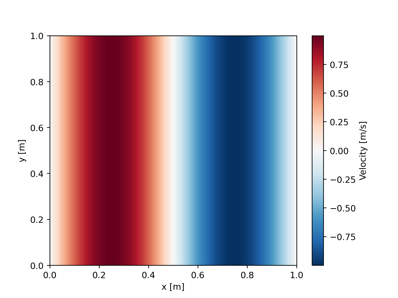
u = sw.FieldVariable(mset, name="u", long_name="Velocity", units="m/s")
X, Y = u.get_mesh()
u.arr = ncp.sin(2 * ncp.pi * X)

# Convert the entire field variable to a DataArray and plot it
u.xr.plot()

Converting a slice

import fridom.shallowwater as sw

grid = sw.grid.cartesian.Grid(N=(256,256), L=(1,1), periodic_bounds=(True, True))
mset = sw.ModelSettings(grid=grid)
mset.setup()

ncp = sw.config.ncp
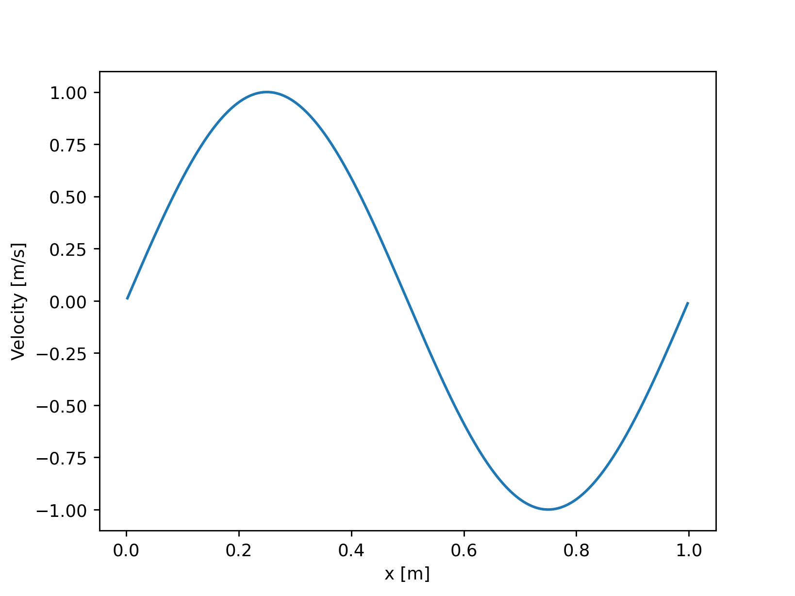
u = sw.FieldVariable(mset, name="u", long_name="Velocity", units="m/s")
X, Y = u.get_mesh()
u.arr = ncp.sin(2 * ncp.pi * X)

# Convert a slice of the field variable to a DataArray and plot it
u.xrs[:, 0].plot()

Tip

If you are working with 3D field variables, you can plot a section of the field in a 2D plot by using the .xrs method with two slices:

u.xrs[:, :, 0].plot()  # plot the z=0 section

You may wonder why we have the .xrs method if you can achieve the same result using the .sel method in xarray. The reason lies in performance. For example, if the array lies on the GPU, it must first be copied to the CPU before being converted into an xarray DataArray. This process is obviously faster when only a part of the array needs to be converted.

Note

The xarray conversion is not compatible when running the framework in parallel.

Differentiation and Interpolation#

When modeling partial differential equations, one is often interested in the derivatives of field variables. Simple partial derivatives can be calculated using the diff method. The method takes as arguments the axis along which the derivative should be computed and the order of the derivative.

Differentiation#

import matplotlib.pyplot as plt
import fridom.shallowwater as sw

grid = sw.grid.cartesian.Grid(N=(256,256), L=(1,1), periodic_bounds=(True, True))
mset = sw.ModelSettings(grid=grid)
mset.setup()

ncp = sw.config.ncp
u = sw.FieldVariable(mset, name="u")
X, Y = u.get_mesh()
u.arr = ncp.sin(2 * ncp.pi * X)

# Calculate the first derivative in the x-direction
du_dx = u.diff(axis=0, order=1)

u.xrs[:, 0].plot(label="u")
du_dx.xrs[:, 0].plot(label="du/dx")
plt.legend()

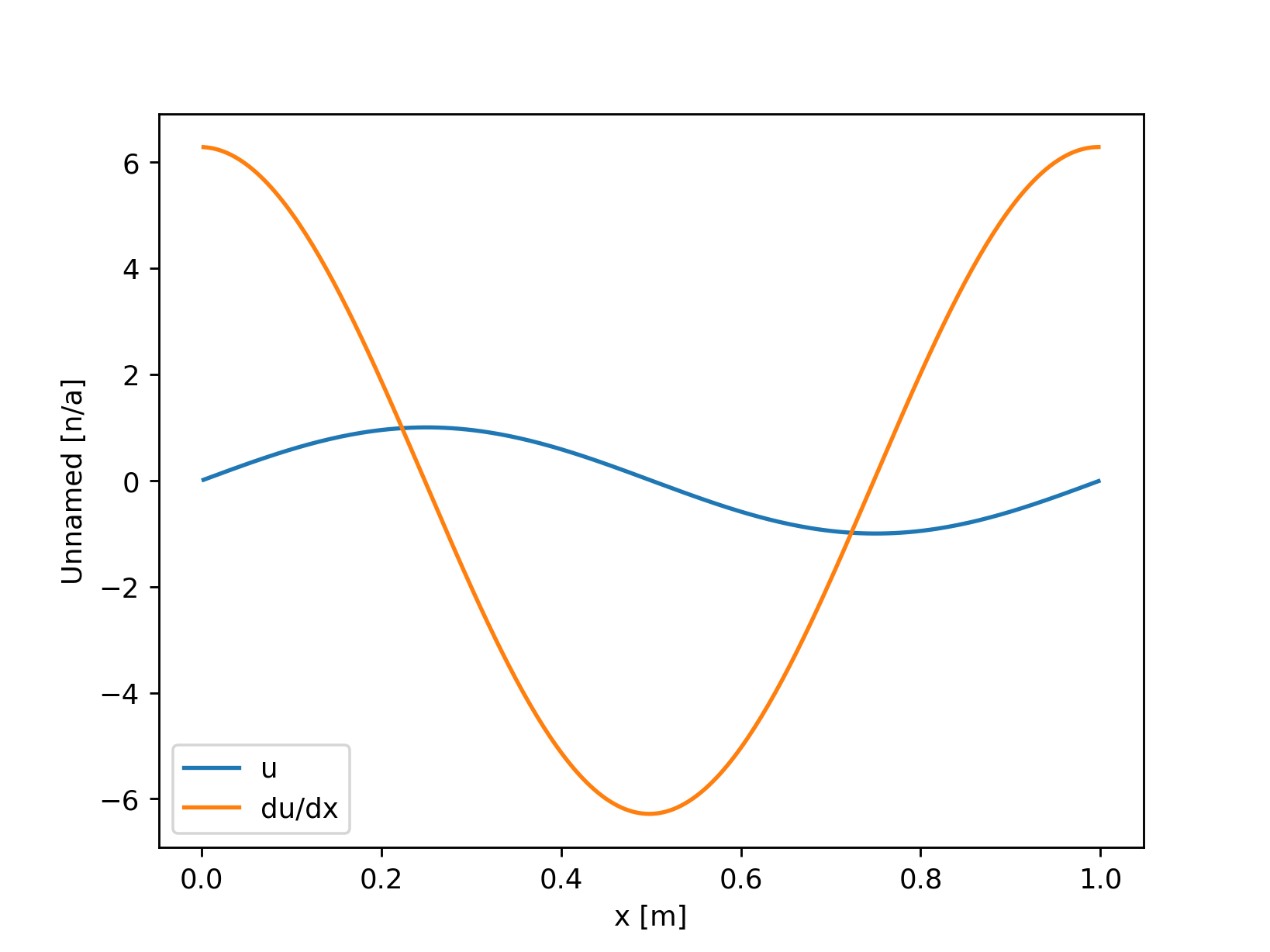
How these derivatives are calculated depends on the type of grid being used. For the Cartesian grid in this example, the derivative is calculated using forward and backward differences. Here, the position of the field variable becomes important. If the field is located at the CENTER in a given direction, the first derivative is computed using a forward difference, and the resulting field is located at the cell FACE. Conversely, if the field is located on the FACE, a backward difference is used to compute the derivative.

Let’s review the positions of the fields from the above example:

print(f"u: {u.position}")
print(f"du_dx: {du_dx.position}")

In some cases, you might want to interpolate a field from one position to another. This can be achieved using the interpolate method, which takes as its argument the position to which the field should be interpolated.

Interpolation#

du_dx_center = du_dx.interpolate(u.position)

The interpolation method used depends on the grid and the underlying interpolation module. In this example, linear interpolation is performed. However, other interpolation methods of higher order are available as well.

Finally, let’s introduce a few useful differentiation functions, all of which are based on the diff method:

Useful differentiation functions#

# Calculate the gradient of a field variable
grad = u.grad()  # returns a list of field variables

# Calculate the Laplacian of a field variable
lap = u.laplacian()

Flat Axes#

So far, we have only considered field variables that have the same dimensions as the grid. However, it is also possible to create field variables that do not extend in certain directions. This can be useful, for instance, when applying 2D surface forcing in a 3D domain or when creating a vertical profile. To achieve this, you can use the topo argument, which is a list of booleans. If topo is True in a given direction, the field variable has an extent in that direction. If topo is False, the field variable has no extent in that direction.

Consider the following example, in which we create a 2D field variable that has an extent in the x-direction but not in the y-direction:

Flat axes#

import fridom.shallowwater as sw

grid = sw.grid.cartesian.Grid(N=(256,256), L=(1,1), periodic_bounds=(True, True))
mset = sw.ModelSettings(grid=grid)
mset.setup()

u = sw.FieldVariable(mset, name="u", topo=[True, False])

If you add this field to a field variable that extends in all directions, the result will be a field variable that extends in all directions. The field variable without extent in a particular direction is assumed to be constant along that direction:

Adding flat axes#

import fridom.shallowwater as sw

grid = sw.grid.cartesian.Grid(N=(256,256), L=(1,1), periodic_bounds=(True, True))
mset = sw.ModelSettings(grid=grid)
mset.setup()

u = sw.FieldVariable(mset, name="v")
v = sw.FieldVariable(mset, name="u", topo=[True, False])

print(u.arr.shape)  # (258, 258)
print(v.arr.shape)  # (258, 1)

u += 1.0
v += 9.0
w = u + v  # w is now 10 everywhere

Note

The number of grid points in the extended directions is 258 and not 256 because the field variable is extended by one grid pointp in each direction to account for the halo regions.

Boundary Conditions#

Warning

Boundary conditions are still under development and are likely to change in the future.

Boundary conditions are particularly important for spectral methods on non-periodic grids. The type of boundary condition can be set individually for each direction. The possible boundary conditions are:

NEUMANN: \(\partial_n u = 0\) (zero normal derivative at the boundary)
DIRICHLET: \(u = 0\) (zero value at the boundary)

By default, all boundaries are set to NEUMANN. They can be customized using the bc_types argument in the field variable class:

Boundary conditions#

import fridom.shallowwater as sw

grid = sw.grid.cartesian.Grid(N=(256,256), L=(1,1), periodic_bounds=(True, True))
mset = sw.ModelSettings(grid=grid)
mset.setup()

NEUMANN = sw.grid.BCType.NEUMANN
DIRICHLET = sw.grid.BCType.DIRICHLET

# u should be zero at the x-boundaries and have zero normal derivative at the y-boundaries
u = sw.FieldVariable(mset, name="u", bc_types=(DIRICHLET, NEUMANN))

Summary#

In this tutorial, we explored how to work with field variables in the FRIDOM framework. We began by creating a field variable and learned how to manipulate its data using arithmetic operations, built-in methods, and numpy functions. We also discussed positioning of field variables on staggered and non-staggered grids, showing how to define a variable’s location on the grid and how this affects derivative computations.

We demonstrated how to utilize xarray to convert field variables for efficient plotting, either converting the entire variable or just a slice for better performance. We then covered calculating derivatives of field variables using the diff method and how the grid type and variable position impact these calculations. Interpolation between positions was shown using the interpolate method, and we provided additional useful differentiation functions like grad and laplacian.

The tutorial also discussed handling flat axes when a field variable does not extend in certain grid dimensions, which is particularly useful for applying surface forcing or creating vertical profiles. Lastly, we briefly introduced boundary conditions, showing how they can be set for different grid directions.

With these tools and techniques, you now have a foundational understanding of how to create, manipulate, analyze, and visualize field variables in FRIDOM, equipping you to create own custom initial conditions, which we will cover in the next tutorial.

Field Variables and Plotting

Contents

Field Variables and Plotting#

Creating Field Variables#

Manipulating Field Variables#

Arithmetic Operations#

Field Variable Methods#

Apply Numpy Functions#

Position of Field Variables#

Plotting Field Variables with Xarray#

Differentiation and Interpolation#

Flat Axes#

Boundary Conditions#

Summary#