VectorField

class fridom.framework.vector_field.VectorField(mset: ModelSettingsBase, field_list: list[ScalarField] | OrderedDict[str, ScalarField] | None = None, vector_dim: int | None = None, **kwargs: any)

Bases: FieldBase

A vector mapping from grid space to the vector space.

Description

A vector field essentially is a list of scalar fields, one for each component of the vector field. This class provides additional methods for vector operations such as dot product, or differential operators like divergence.

Parameters

msetfr.ModelSettingsBase

The model settings object.

field_listlist[fr.ScalarField] | OrderedDict[str, fr.ScalarField] | None

The list of scalar fields that make up the vector field.

vector_dimint | None

The vector dimension. If None, it is set to the length of field_list.

**kwargsany

Additional keyword arguments to pass to the scalar fields.

__init__(mset: ModelSettingsBase, field_list: list[ScalarField] | OrderedDict[str, ScalarField] | None = None, vector_dim: int | None = None, **kwargs: any) → None

Methods

__init__(mset[, field_list, vector_dim])
abs()	Map the field by taking the absolute value (\(|f|\)).
apply_elementwise(vector_field, op)	Apply an operation elementwise to the vector field.
apply_water_mask()	Apply a water mask to the field.
conj()	Compute the complex conjugate.
cumulative_integral(axis[, direction])	Compute the cumulative integral along an axis.
diff(axis[, order])	Compute the partial derivative along an axis.
div()	Compute the divergence.
dot(other)	Compute the dot product with another field.
extend(topo)	Extend the field in the specified directions.
fft([padding])	Perform a Fast Fourier Transform (FFT) on the field.
from_netcdf(mset, path)	Create a field from a NetCDF file.
from_xarray(mset, ds)	Create a field from an xarray object.
grad([axes])	Compute the gradient.
has_nan()	Check if the field contains NaN values.
ifft([padding])	Perform an Inverse Fast Fourier Transform (IFFT) on the field.
integrate([axes])	Global integral of the Field in specified axes.
laplacian([axes])	Compute the Laplacian.
max([axes])	Maximum value of the Field over the whole domain.
mean([axes])	Global mean of the Field in specified axes.
min([axes])	Minimum value of the Field over the whole domain.
norm_l2()	Calculate the L2 norm of the field.
norm_of_diff(other)	Norm of difference between two vector fields.
project(p_vec, q_vec)	Project a Vector Field onto a (spectral) vector.
set_random([seed])	Set the field to random values.
sum([axes])	Sum of the Field over the whole domain in the specified axes.
sync()	Synchronize the field across all MPI ranks and apply boundary conditions.
to_netcdf(path)	Save the field to a NetCDF file.

Attributes

field_list	The list of scalar fields.
fields	The dictionary of scalar fields.
grid	The grid object.
info	Dictionary with information about the field.
is_constant	Flag indicating whether the field is constant.
is_spectral	Flag indicating whether the field is in spectral space.
mset	The model settings.
vector_dim	The vector dimension.
xr	The xarray representation of the field.
xrs	Convert a slice of the field to an xarray object.

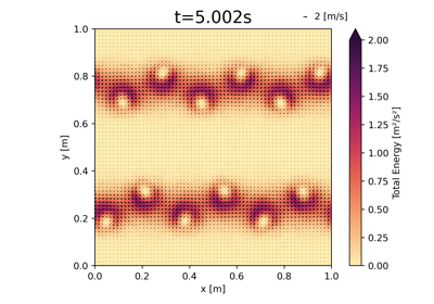
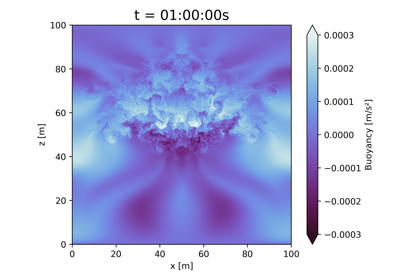
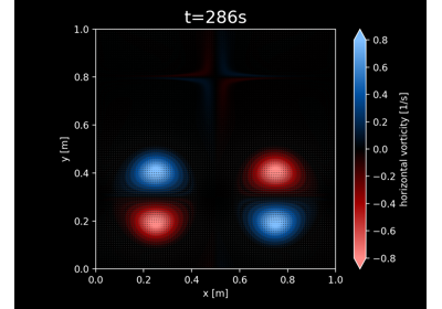
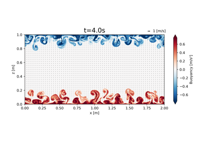
Examples using fridom.framework.VectorField

Barotropic Jet

Barotropic Jet

Convection and Closures

Convection and Closures

Dancing Eddies

Dancing Eddies

Rayleigh-Bénard Convection

Rayleigh-Bénard Convection

Rayleigh-Taylor Instability

Rayleigh-Taylor Instability

Single Internal Wave

Single Internal Wave

Symmetric Instability

Symmetric Instability

Tracers and Eddies

Tracers and Eddies

Reflecting Wave Package

Reflecting Wave Package

Barotropic Instability.

Barotropic Instability.

Equatorial Waves.

Equatorial Waves.

fft(padding: FFTPadding = FFTPadding.NOPADDING) → T

Perform a Fast Fourier Transform (FFT) on the field.

Description

Computes the Fast Fourier Transform (FFT) of the field. The padding parameter can be used to specify the zero-padding strategy.

Parameters

paddingfr.grid.FFTPadding

The padding strategy.

Returns

FieldBase

The FFT of the field.

ifft(padding: FFTPadding = FFTPadding.NOPADDING) → T

Perform an Inverse Fast Fourier Transform (IFFT) on the field.

Description

Computes the Inverse Fast Fourier Transform (IFFT) of the field. The padding parameter can be used to specify the zero-padding strategy.

Parameters

paddingfr.grid.FFTPadding

The padding strategy.

Returns

FieldBase

The IFFT of the field.

project(p_vec: T, q_vec: T) → T

Project a Vector Field onto a (spectral) vector.

Description

The projection of the vector \(\boldsymbol{z}\) on a P-Vector \(\boldsymbol{z}\) and a Q-Vector \(\boldsymbol{q}\) is defined as:

\[\boldsymbol{z} = \boldsymbol{q} \cdot \left( \boldsymbol{z} \cdot \boldsymbol{p} \right)\]

The projection is done in spectral space. All vectors are transformed to spectral space before the projection and transformed back to physical space if necessary.

Parameters

p_vecVectorField

the projection vector \(\boldsymbol{p}\)

q_vecVectorField

the polarization vector \(\boldsymbol{q}\)

Returns

VectorField

The projected vector field \(\boldsymbol{z}\)

sync() → T

Synchronize the field across all MPI ranks and apply boundary conditions.

Description

This method synchronizes the field across all MPI ranks and applies the boundary conditions. This is necessary to ensure that the ghost cells are up-to-date. This method changes the field in-place, but also returns the synchronized field.

Returns

FieldBase

The synchronized field.

apply_water_mask() → T

Apply a water mask to the field.

Description

A water mask is a binary field that indicates which cells are water (active) and which are land (inactive). This method applies the water mask to the field. The field is changed in-place.

Returns

FieldBase

The field with the water mask applied.

has_nan() → bool

Check if the field contains NaN values.

Returns

bool

Flag indicating whether the field contains NaN values.

set_random(seed: int = 1234) → T

Set the field to random values.

Description

This method sets the field to random values. If the field is in spectral space, the random values are complex.

Parameters

seedint

The seed for the random number generator.

Returns

FieldBase

The field with random values.

diff(axis: int, order: int = 1) → T

Compute the partial derivative along an axis.

\[\partial_i^n f\]

with axis \(i\) and order \(n\).

Parameters

axisint

The axis along which to differentiate.

orderint

The order of the derivative. Default is 1.

Returns

fr.ScalarField | fr.VectorField | fr.TensorField

The derivative of the field along the specified axis.

grad(axes: list[int] | None = None) → TensorField

Compute the gradient.

\[\begin{split}\nabla f = \begin{pmatrix} \partial_1 f \\ \dots \\ \partial_n f \end{pmatrix}\end{split}\]

Parameters

axeslist[int] | None (default is None)

The axes along which to compute the gradient. If None, the gradient is computed along all axes.

Returns

fr.VectorField | fr.TensorField

The gradient of the field along the specified axes. The list contains the gradient components along each axis. Axis which are not included in axes will have a value of None. E.g. for a 3D grid, diff.grad(f, axes=[0, 2]) will return [df/dx, None, df/dz].

laplacian(axes: tuple[int] | None = None) → T

Compute the Laplacian.

\[\nabla^2 f = \sum_{i=1}^n \partial_i^2 f\]

Parameters

axestuple[int] | None (default is None)

The axes along which to compute the Laplacian. If None, the Laplacian is computed along all axes.

Returns

fr.ScalarField | fr.VectorField | fr.TensorField

The Laplacian of the field.

div() → ScalarField

Compute the divergence.

\[\nabla \cdot f = \sum_{i=1}^n \partial_i f\]

Returns

fr.ScalarField | fr.VectorField

The divergence of the field.

cumulative_integral(axis: int, direction: Literal['forward', 'backward'] = 'forward') → VectorField

Compute the cumulative integral along an axis.

Description

The cumulative integral computes the integral starting at one end of the domain and accumulates the integral along the specified axis. The integral is computed in either the forward or backward direction.

Forward integral:

\[\int_{x_0}^{x} f(x') dx'\]

with axis \(x\) and \(x_0\) the lower bound of the domain.

Backward integral:

\[\int_{x}^{x_1} f(x') dx'\]

with axis \(x\) and \(x_1\) the upper bound of the domain.

Parameters

axisint

The axis along which to integrate.

directionstr (default is “forward”)

The direction of the integration. Can be “forward” or “backward”.

Returns

fr.ScalarField | fr.VectorField | fr.TensorField

The cumulative integral of the field along the specified axis.

property xr: xr.Dataset

The xarray representation of the field.

Returns

xr.DataArray | xr.Dataset

The xarray representation of the field.

property xrs: fr.utils.SliceableAttribute[xr.Dataset]

Convert a slice of the field to an xarray object.

Description

This method returns a sliceable attribute that allows to convert a slice of the field to an xarray object. This is useful when dealing with large fields and only a subset of the data is needed. For example, the top region of the field.

classmethod from_xarray(mset: fr.ModelSettingsBase, ds: xr.Dataset) → T

Create a field from an xarray object.

Description

This method creates a field from an xarray object. The model settings are required to create the field.

Parameters

msetfr.ModelSettingsBase

The model settings.

dsxr.DataArray | xr.Dataset

The xarray object.

Returns

FieldBase

The field.

property info: dict

Dictionary with information about the field.

property fields: OrderedDict[str, ScalarField]

The dictionary of scalar fields.

property field_list: list[ScalarField]

The list of scalar fields.

property vector_dim: int

The vector dimension.

property is_spectral: bool

Flag indicating whether the field is in spectral space.

property is_constant: bool

Flag indicating whether the field is constant.

extend(topo: tuple[bool]) → T

Extend the field in the specified directions.

Description

This method extends the field in the specified directions. The field can be extended in any direction, but it cannot be shrunk. This means that if the field is extended in a direction, it has to be extended in all directions. Values in the extended directions are copied from the original field, such that:

\[f_{\text{new}}(x, y, z) = f_{\text{old}}(x, y)\]

where \(f_{\text{new}}\) is the new field extended in (x, y, z), and \(f_{\text{old}}\) is the old field, extended in (x, y).

Parameters

topotuple[bool]

The new topology of the field.

Returns

FieldBase

The extended field.

Raises

ValueError

If the field is shrunk in any direction.

sum(axes: tuple[int] | None = None) → T

Sum of the Field over the whole domain in the specified axes.

Description

This method computes the sum of the Field over the whole domain (across all processes) in the specified axes. If no axes are specified, the sum is computed over all axes.

Note

We recommend using the f.integrate() method to integrate the field in certain directions. The integrate() method takes the grid spacing into account while the sum() method does not.

Parameters

axestuple[int] | None

The axes to sum over. If None, sum over all axes.

Returns

FieldBase

The sum of the field. The returned field has no extend in the specified axes.

max(axes: tuple[int] | None = None) → T

Maximum value of the Field over the whole domain.

Description

This method computes the maximum value of the Field over the whole domain (across all processes) in the specified axes. If no axes are specified, the maximum is computed over all axes.

Parameters

axestuple[int] | None

The axes to compute the maximum over. If None, compute the maximum over all axes.

Returns

FieldBase

The maximum value of the Field over the specified axes. The returned field has no extend in the specified axes.

min(axes: tuple[int] | None = None) → T

Minimum value of the Field over the whole domain.

Description

This method computes the minimum value of the Field over the whole domain (across all processes) in the specified axes. If no axes are specified, the minimum is computed over all axes.

Parameters

axestuple[int] | None

The axes to compute the minimum over. If None, compute the minimum over all axes.

Returns

FieldBase

The minimum value of the Field over the specified axes. The returned field has no extend in the specified axes.

integrate(axes: tuple[int] | None = None) → T

Global integral of the Field in specified axes.

Description

Computes the global integral of the Field in the specified axes:

\[\sum_{i} \int_{x_i} f(\boldsymbol{x}) dx_i\]

If no axes are specified, the integral is computed over all axes.

Parameters

axestuple[int] | None

The axes to integrate over. If None, integrate over all axes.

Returns

FieldBase

The integral of the Field over the specified axes.

mean(axes: tuple[int] | None = None) → T

Global mean of the Field in specified axes.

Description

Computes the global mean of the Field in the specified axes:

\[\frac{\sum_{i} \int_{x_i} f(\boldsymbol{x}) dx_i} {\sum_{i} \int_{x_i} dx_i}\]

If no axes are specified, the mean is computed over all axes.

Parameters

axestuple[int] | None

The axes to compute the mean over. If None, compute the mean over all axes.

Returns

FieldBase

The mean of the Field over the specified axes.

norm_of_diff(other: VectorField) → float

Norm of difference between two vector fields.

Description

The norm of difference computes the normalized difference between two vector fields \(\boldsymbol{z}\) and \(\boldsymbol{z}'\). It is defined as:

\[2 \frac{||\boldsymbol{z} - \boldsymbol{z}'||} {||\boldsymbol{z}|| + ||\boldsymbol{z}'||}\]

where \(||\cdot||\) is the L2 norm of the vector field. The norm of difference is in the range [0, 2].

Parameters

otherVectorField

The other vector field to compare with

Returns

float

The norm of difference between the two vector fields

dot(other: ScalarField | VectorField | TensorField) → ScalarField | VectorField | T

Compute the dot product with another field.

Parameters

otherFieldBase

The other field.

Returns

FieldBase

The dot product.

Description

Computes the dot product with another field. The dot product is defined as

\[f \cdot g^*\]

where \(f\) and \(g\) are the fields and \(^*\) denotes the complex conjugate.

The return value depends on the type of the fields. The following table shows the possible return values:

Field Type	Field Type	Return Type
ScalarField	ScalarField	ScalarField
ScalarField	VectorField	VectorField
ScalarField	TensorField	TensorField
VectorField	ScalarField	VectorField
VectorField	VectorField	ScalarField
VectorField	TensorField	Error
TensorField	ScalarField	TensorField
TensorField	VectorField	VectorField
TensorField	TensorField	TensorField

conj() → T

Compute the complex conjugate.

Returns

FieldBase

The complex conjugate. If the field is real, the field itself is returned.

abs() → T

Map the field by taking the absolute value (\(|f|\)).

Returns

FieldBase

The absolute value of the field.

static apply_elementwise(vector_field: T, op: Callable[[ScalarField], ScalarField]) → T

Apply an operation elementwise to the vector field.

Description

This method applies an operation elementwise to each scalar field in the vector field and returns a new vector field with the modified fields.

Parameters

vector_fieldVectorField

The vector field to apply the operation to.

opCallable[[fr.ScalarField], fr.ScalarField]

The operation to apply to each scalar field. Should take a scalar field as input and return a scalar field.

Returns

VectorField

The new vector field with the modified fields