State

class fridom.shallowwater.State(mset: ModelSettings, **kwargs: any)

Bases: VectorField

State vector of the 2D shallow water model.

Description

The default scalar fields of the state vector are:

• u: Velocity in the x-direction.

• v: Velocity in the y-direction.

• p: Pressure field, with \(p = g \eta\), where \(\eta\) is the

free surface elevation.

__init__(mset: ModelSettings, **kwargs: any) → None

Methods

__init__(mset, **kwargs)
abs()	Map the field by taking the absolute value (\(|f|\)).
apply_elementwise(vector_field, op)	Apply an operation elementwise to the vector field.
apply_water_mask()	Apply a water mask to the field.
conj()	Compute the complex conjugate.
cumulative_integral(axis[, direction])	Compute the cumulative integral along an axis.
diff(axis[, order])	Compute the partial derivative along an axis.
div()	Compute the divergence.
dot(other)	Compute the dot product with another field.
extend(topo)	Extend the field in the specified directions.
fft([padding])	Perform a Fast Fourier Transform (FFT) on the field.
from_netcdf(mset, path)	Create a field from a NetCDF file.
from_xarray(mset, ds)	Create a field from an xarray object.
grad([axes])	Compute the gradient.
has_nan()	Check if the field contains NaN values.
ifft([padding])	Perform an Inverse Fast Fourier Transform (IFFT) on the field.
integrate([axes])	Global integral of the Field in specified axes.
laplacian([axes])	Compute the Laplacian.
max([axes])	Maximum value of the Field over the whole domain.
mean([axes])	Global mean of the Field in specified axes.
min([axes])	Minimum value of the Field over the whole domain.
norm_l2()	Calculate the L2 norm of the field.
norm_of_diff(other)	Norm of difference between two vector fields.
project(p_vec, q_vec)	Project a Vector Field onto a (spectral) vector.
set_random([seed])	Set the field to random values.
sum([axes])	Sum of the Field over the whole domain in the specified axes.
sync()	Synchronize the field across all MPI ranks and apply boundary conditions.
to_netcdf(path)	Save the field to a NetCDF file.

Attributes

cfl	The CFL number.
ekin	Vertically integrated kinetic energy.
epot	Vertically integrated kinetic energy.
etot	The total energy.
field_list	The list of scalar fields.
fields	The dictionary of scalar fields.
grid	The grid object.
info	Dictionary with information about the field.
is_constant	Flag indicating whether the field is constant.
is_spectral	Flag indicating whether the field is in spectral space.
local_rossby_number	Local Rossby number.
mset	The model settings.
p	Pressure \(p\).
pot_vort	Scaled potential vorticity field.
rel_vort	Relative vorticity.
spectral_ekin	Spectral kinetic energy density.
tracers	The tracer fields.
u	Velocity in the x-direction.
v	Velocity in the y-direction.
vector_dim	The vector dimension.
velocity	Velocity vector.
xr	The xarray representation of the field.
xrs	Convert a slice of the field to an xarray object.

Examples using fridom.shallowwater.State

Barotropic Instability.

Barotropic Instability.

Equatorial Waves.

Equatorial Waves.

property u: ScalarField

Velocity in the x-direction.

property v: ScalarField

Velocity in the y-direction.

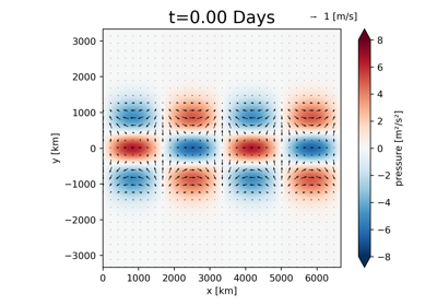
property p: ScalarField

Pressure \(p\).

Description

The pressure field is defined as

\[p = g \eta\]

where \(\eta\) is the free surface elevation and \(g\) is the gravity acceleration.

property velocity: VectorField

Velocity vector.

property tracers: VectorField

The tracer fields.

property ekin: ScalarField

Vertically integrated kinetic energy.

\[E_{\text{kin}} = \frac{Ro^2}{2} h_{\text{full}} (u^2 + v^2)\]

with

\[h_{\text{full}} = c^2 + Ro p\]

Note:

The energy is scaled with the gravity acceleration g.

property epot: ScalarField

Vertically integrated kinetic energy.

\[E_{\text{pot}} = \frac{1}{2} h_{\text{full}}^2\]

with

\[h_{\text{full}} = c^2 + Ro p\]

Note:

The energy is scaled with the gravity acceleration g.

property etot: ScalarField

The total energy.

\[E_{tot} = E_{kin} + E_{pot}\]

property spectral_ekin: ScalarField

Spectral kinetic energy density.

\[S_{\text{kin}} = \frac{1}{2} (|\hat{u}|^2 + |\hat{v}|^2)\]

property rel_vort: ScalarField

Relative vorticity.

\[\zeta = \partial_x v - \partial_y u\]

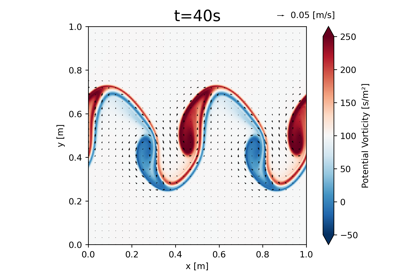
property pot_vort: ScalarField

Scaled potential vorticity field.

\[Q = \frac{\zeta + f \right}{c^2 + Ro p}\]

where \(f\) is the Coriolis parameter, and \(\zeta\) is the relative vorticity.

property local_rossby_number: ScalarField

Local Rossby number.

\[Ro_\text{local} = Ro \, \frac{\zeta_z}{f_0}\]

where \(Ro\) is the Rossby number, \(\zeta_z\) is the vertical component of the relative vorticity, and \(f_0\) is the Coriolis parameter.

property cfl: ScalarField

The CFL number.

\[CFL = \max \left\{ \frac{u}{\Delta x}, \frac{v}{\Delta y} \right\} \Delta t\]

where \(\Delta t\) is the time step and \(\Delta x\) is the grid spacing.