
The State Vector and Initial Conditions#
In the last tutorial, we saw that scalar fields in fridom are analogous to DataArrays in xarray.
In this tutorial, we will introduce the state vector, which corresponds to Datasets in xarray.
Essentially, the state vector is a container for scalar fields, offering additional functionality useful for analysis.
For example, it provides methods to calculate quantities like energy or vorticity.
Let’s take a look at the state vector in two different model setups:
import fridom.shallowwater as sw

# Create the grid and model settings
grid = sw.grid.cartesian.Grid(N=(256, 256), L=(1, 1), periodic_bounds=(True, True))
mset = sw.ModelSettings(grid=grid)
mset.setup()

# Create the state vector
z = sw.State(mset)
print(z)
Output
State(
  u=u - velocity  [m/s],
  v=v - velocity  [m/s],
  p=pressure  [m²/s²],
)
import fridom.nonhydro as nh

# Create the grid and model settings
grid = nh.grid.cartesian.Grid(N=(256, 256, 16), L=(1, 1, 1), periodic_bounds=(True, True, False))
mset = nh.ModelSettings(grid=grid)
mset.setup()

# Create the state vector
z = nh.State(mset)
print(z)
Output
State(
  u=u - velocity  [m/s],
  v=v - velocity  [m/s],
  w=w - velocity  [m/s],
  b=Buoyancy  [m/s²],
)
As you can see, the state vector of the shallow water model contains the velocities in the x and y directions and the pressure. In contrast, the 3D nonhydrostatic model includes the velocities in x, y, and z directions, as well as the buoyancy.
You might wonder why the pressure is not included in the 3D nonhydrostatic model. This is because pressure in the 3D nonhydrostatic model is not a prognostic variable, but rather a diagnostic one. Most systems of partial differential equations can be written in the following general form:
where \(\boldsymbol{z}\) represents the prognostic state vector, and \(\boldsymbol{r}\) stands for the diagnostic variables. \(\boldsymbol{f}\) is the tendency function, and \(g\) are additional equations to close the system. For the nonhydrostatic incompressible Navier-Stokes equations, \(g\) would correspond to the continuity equation. If you take a closer look at the system of equations governing the 3D nonhydrostatic model, you’ll notice there is no tendency equation for pressure. Hence, the pressure should not be included in the state vector.
We will explore the diagnostic vector \(\boldsymbol{r}\) in more detail in this tutorial, where you will learn how to access pressure in the nonhydrostatic model. For now, you just need to remember that the state vector only contains the prognostic variables.
Let’s explore how to work with the state vector:
Working with the State Vector#
In the examples above, you have already seen how to create a state vector and that it contains scalar fields. When initializing a state vector, all scalar fields are set to zero. This is typically not a very interesting state, so you often initialize the state vector with specific initial conditions. To do this, you first need to know how to access the scalar fields in the state vector. The following examples show two ways to access scalar fields: Either as a dictionary or as an attribute:
import fridom.shallowwater as sw

# Create the grid and model settings
grid = sw.grid.cartesian.Grid(N=(256, 256), L=(1, 1), periodic_bounds=(True, True))
mset = sw.ModelSettings(grid=grid)
mset.setup()

# Create the state vector
z = sw.State(mset)

# Add 1.0 to the u scalar field
z["u"] += 1.0
import fridom.shallowwater as sw

# Create the grid and model settings
grid = sw.grid.cartesian.Grid(N=(256, 256), L=(1, 1), periodic_bounds=(True, True))
mset = sw.ModelSettings(grid=grid)
mset.setup()

# Create the state vector
z = sw.State(mset)

# Add 1.0 to the u scalar field
z.u += 1.0
In both cases, 1.0 is added to the u scalar field. While the attribute approach is a bit shorter and therefore quicker to write, it requires that the scalar fields in the state vector are defined as properties. Later in this tutorial, we will see how to add custom scalar fields to the state vector. These will not be defined as properties and can only be accessed via the dictionary approach.
Now that you know how to access the scalar fields in the state vector, you can use the methods learned in the previous tutorial to modify the state vector as needed. Additionally, there are methods you can apply to the state vector that will be executed on all its scalar fields. This can be particularly useful in cases where you want to add two state vectors, square all scalar fields, apply a Fourier transform to all fields, and so on:
import fridom.shallowwater as sw

# Create the grid and model settings
grid = sw.grid.cartesian.Grid(N=(256, 256), L=(1, 1), periodic_bounds=(True, True))
mset = sw.ModelSettings(grid=grid)
mset.setup()

# Create the state vector
z1 = sw.State(mset)
z2 = sw.State(mset)

# Multiply the state vector by 2
z1 *= 2

# Add the two state vectors together
z3 = z1 + z2  # z3 will inherit attributes from z1

# Apply Fourier transform to the state vector
z1_hat = z1.fft()
z1_back = z1_hat.ifft()

# Synchronize halo regions of all fields
z1 = z1.sync()
Xarray Conversion and Plotting#
Similar to the scalar fields, state vectors also have the properties .xr and .xrs for converting the state vector into an xarray Dataset.
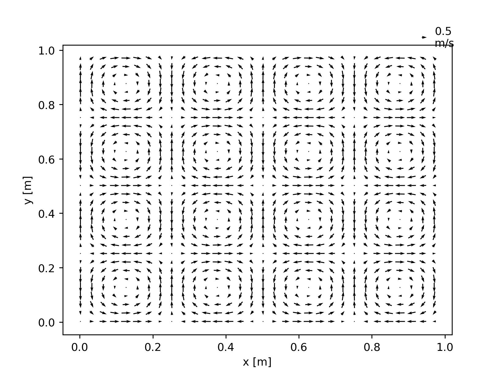
This can be particularly useful when creating a quiver plot of the velocity field:
import fridom.shallowwater as sw

# Create the grid and model settings
grid = sw.grid.cartesian.Grid(N=(256, 256), L=(1, 1), periodic_bounds=(True, True))
mset = sw.ModelSettings(grid=grid)
mset.setup()

# Create the state vector
z = sw.State(mset)

# Create a velocity field
ncp = sw.config.ncp
X, Y = z.u.get_mesh()
z.u.arr = ncp.sin(4 * ncp.pi * X) * ncp.cos(4 * ncp.pi * Y)
z.v.arr = -ncp.cos(4 * ncp.pi * X) * ncp.sin(4 * ncp.pi * Y)

# Convert the state vector to an xarray dataset and plot the velocity field
z.xrs[::8, ::8].plot.quiver("x", "y", "u", "v")
import fridom.shallowwater as sw

# Create the grid and model settings
grid = sw.grid.cartesian.Grid(N=(256, 256), L=(1, 1), periodic_bounds=(True, True))
mset = sw.ModelSettings(grid=grid)
mset.setup()

# Create the state vector
z = sw.State(mset)

# Create a velocity field
ncp = sw.config.ncp
X, Y = z.u.get_mesh()
z.u.arr = ncp.sin(4 * ncp.pi * X) * ncp.cos(4 * ncp.pi * Y)
z.v.arr = -ncp.cos(4 * ncp.pi * X) * ncp.sin(4 * ncp.pi * Y)

# Convert the state vector to an xarray dataset and plot the velocity field
z.xr.plot.quiver("x", "y", "u", "v")

In the example using the .xr property, the entire state vector is converted into an xarray Dataset, and a quiver plot of the velocities is generated.
Since an arrow is created for each point on the grid, the arrows become indistinguishable, rendering the plot less useful.
To address this, you can reduce the number of grid points converted into the xarray Dataset.
In the example above, we achieve this by only taking every 8th point ([::8, ::8]).
Setting Initial Conditions#
If you want to use a state vector as the initial condition for a model, you can do so by setting the z attribute of the model:
import fridom.shallowwater as sw

# Create the grid and model settings
grid = sw.grid.cartesian.Grid(N=(256, 256), L=(1, 1), periodic_bounds=(True, True))
mset = sw.ModelSettings(grid=grid)
mset.setup()

# Create the state vector
z_ini = sw.State(mset)

# Modify the state vector
# ...

# Create a model (see next tutorial for more details)
model = sw.Model(mset)

# Set state to the model
model.z = z_ini
We will dive deeper into the model itself in the next tutorial. Here, the focus is simply on demonstrating how to use the state vector as an initial condition for a model.
Built-in Initial Conditions#
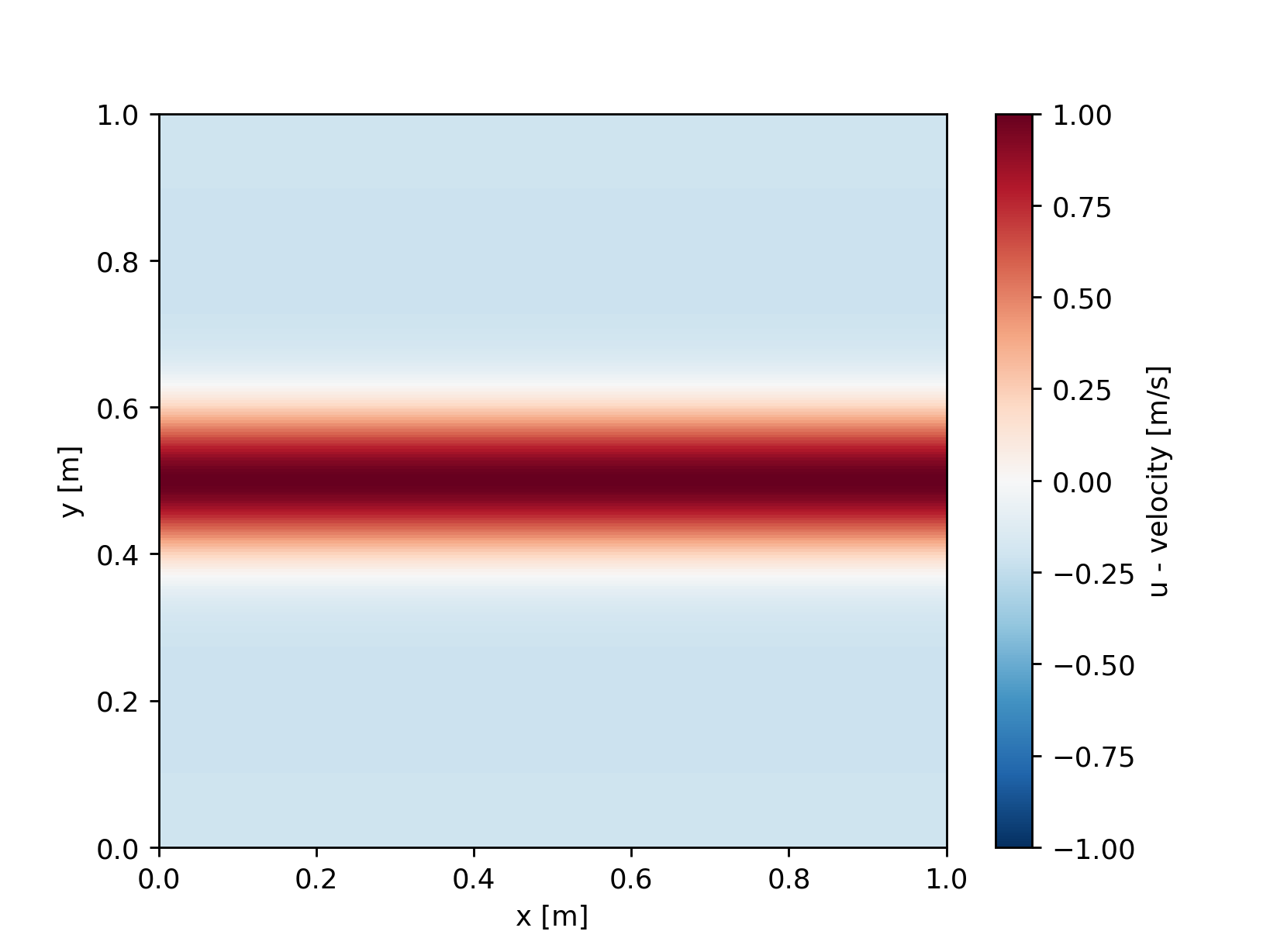
Some models come with built-in initial conditions that you can use. For example, the shallow water model has a built-in Jet initial condition:
import fridom.shallowwater as sw

# Create the grid and model settings
grid = sw.grid.cartesian.Grid(N=(256, 256), L=(1, 1), periodic_bounds=(True, True))
mset = sw.ModelSettings(grid=grid)
mset.setup()

# Create a state vector with the Jet initial condition
z = sw.initial_conditions.Jet(mset, width=0.1, wavenum=2, waveamp=0.05)

z.u.xr.plot()
These initial conditions can be used as building blocks. For instance, it is possible to construct a state as a superposition of different initial conditions.
For a complete list of built-in initial conditions, refer to the API documentation of the respective model. We will now have a look at how to create custom initial conditions. To do so, we create a new class for the initial condition that inherits from the State class.
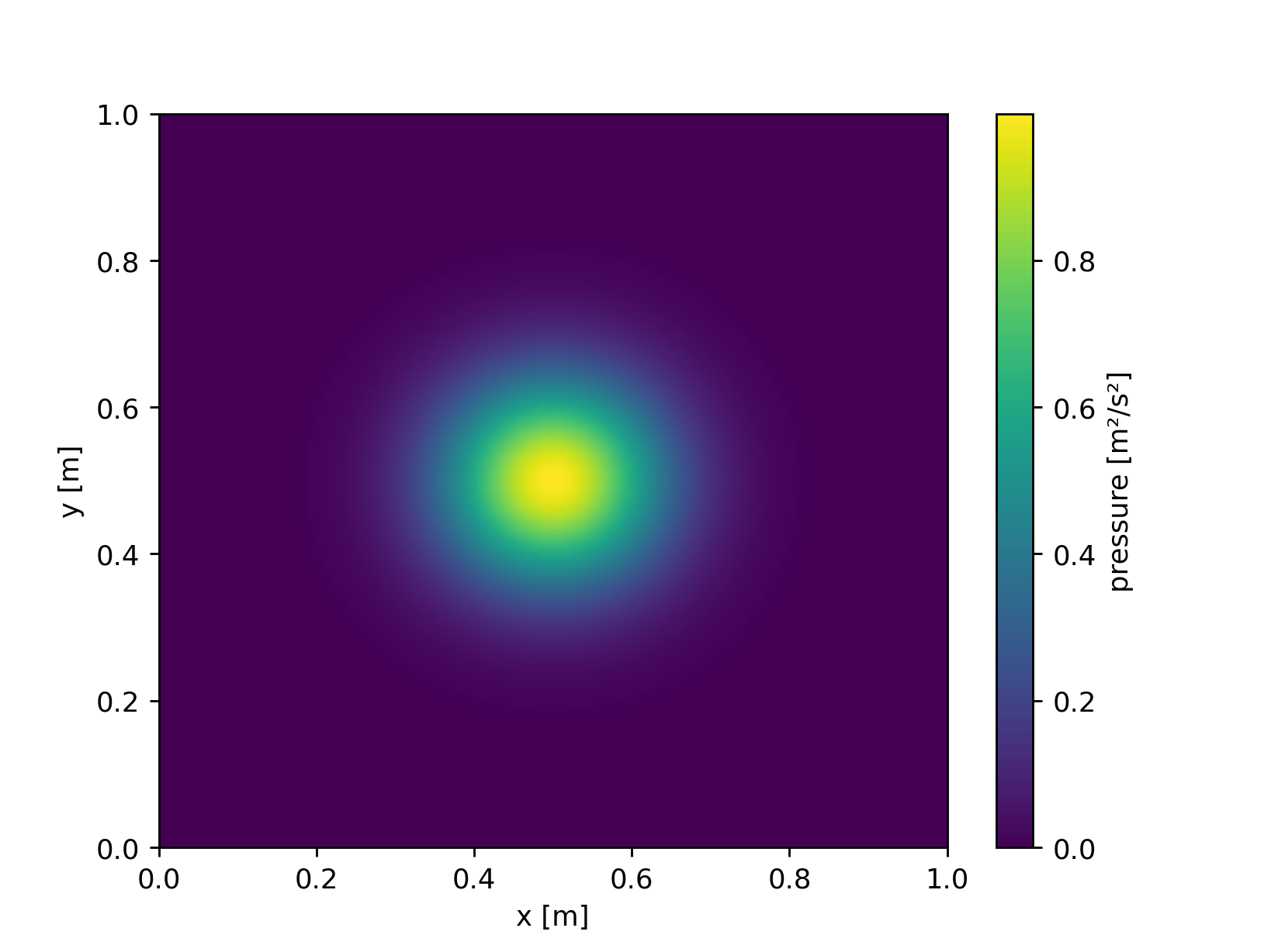
The following example shows how to create a custom initial condition that generates a Gaussian hill in the pressure field:
import fridom.shallowwater as sw

class GaussianPressurePerturbation(sw.State):

    r"""
    Gaussian perturbation in the pressure field.

    Description
    -----------
    This initial condition creates a circular Gaussian hill in the pressure field,
    centered in the middle of the domain. It is defined as:

    .. math::

        p = h \exp\left(-\frac{(x-L_x/2)^2 + (y-L_y/2)^2}{2w^2}\right)

    where :math:`h` is the height of the hill, :math:`w` is the width of the hill,
    and :math:`L_x` and :math:`L_y` are the lengths of the domain in the x and y directions.

    Parameters
    ----------
    mset : ModelSettings
        The model settings object.
    width : float
        The width of the Gaussian hill.
    height : float
        The height of the Gaussian hill. Default is 1.0.

    """

    def __init__(self,
                mset: sw.ModelSettings,
                width: float = 0.1,
                height: float = 1.0) -> None:
        super().__init__(mset)

        x, y = self.p.get_mesh()
        lx, ly = mset.grid.L
        ncp = sw.config.ncp

        self.p.arr = height * ncp.exp(-((x - lx/2)**2 + (y - ly/2)**2) / (2 * width**2))

# Create the grid and model settings
grid = sw.grid.cartesian.Grid(N=(256, 256), L=(1, 1), periodic_bounds=(True, True))
mset = sw.ModelSettings(grid=grid)
mset.setup()

# Create a state vector with the Gaussian Hill initial condition
z = GaussianPressurePerturbation(mset, width=0.1, height=1.0)

z.p.xr.plot()
Tip
Always add a documentation to your initial condition so that other users know how to use it. The example above shows you the structure that such a documentation should have.
Diagnostic Variables#
When working with state vectors, one typically is not only interested in the prognostic variables but also in various diagnostic variables, such as energy or vorticity. To avoid rewriting the same calculations each time you want to compute a quantity like energy, you can make use of the diagnostic variables available within the state vector. It’s best to refer to the API documentation for the state vector of the respective model to see which diagnostic variables are available. For example, in the case of the shallow water model, you can calculate kinetic, potential, and total energy, as well as relative vorticity and potential vorticity. The following example demonstrates how to calculate the potential vorticity of the Jet initial condition:
import fridom.shallowwater as sw

# Create the grid and model settings
grid = sw.grid.cartesian.Grid(N=(256, 256), L=(1, 1), periodic_bounds=(True, True))
mset = sw.ModelSettings(grid=grid)
mset.setup()

# Create a state vector with the Jet initial condition
z = sw.initial_conditions.Jet(mset, width=0.1, wavenum=2, waveamp=0.05)

# Plot the potential vorticity
z.pot_vort.xr.plot()

Adding Custom Scalar Fields to the State Vector#
Warning
FIXME: The functionality has changed, code snippet will no longer work
In most cases, there’s no need to add custom scalar fields to the state vector. However, there are instances where this might be desired. For example, if you want to add tracer scalar fields or additional prognostic variables for turbulence models. These variables are added through the model settings. In the following example, we add the CO₂ concentration as a scalar field:
import fridom.shallowwater as sw

# Create the grid and model settings
grid = sw.grid.cartesian.Grid(N=(256, 256), L=(1, 1), periodic_bounds=(True, True))
mset = sw.ModelSettings(grid=grid)
mset.setup()

# Add the CO2 scalar field to the model settings
mset.add_field_to_state({'name': "co2",
                         'long_name': "CO₂ concentration",
                         'units': "ppm"})

# Create the state vector
z = sw.State(mset)
print(z)
print(z["co2"])
Output
State with fields:
u: u - velocity  [m/s]
v: v - velocity  [m/s]
p: pressure  [m²/s²]
co2: CO₂ concentration  [ppm]

ScalarField
- name: co2
- long_name: CO² concentration
- units: ppm
- is_spectral: False
- position: Position: (<AxisPosition.CENTER: 1>, <AxisPosition.CENTER: 1>)
- topo: [True, True]
- bc_types: (<BCType.NEUMANN: 2>, <BCType.NEUMANN: 2>)
- enabled_flags: []
Note
The dictionary passed to the add_field_to_state method contains the keyword arguments needed for creating a new scalar field.
Scalar fields receive this dictionary as kwargs in their constructor.
Saving and Loading State Vectors#
State vectors can be saved to and loaded from netCDF files. When loading a netCDF file, the model settings object must be passed as a parameter. The following example shows how to save a state vector to a netCDF file and load it back:
import fridom.shallowwater as sw

# Create the grid and model settings
grid = sw.grid.cartesian.Grid(N=(256, 256), L=(1, 1), periodic_bounds=(True, True))
mset = sw.ModelSettings(grid=grid)
mset.setup()

# Create the state vector from the jet initial condition
z = sw.initial_conditions.Jet(mset, width=0.1, wavenum=2, waveamp=0.05)

# Save the state vector to a netCDF file
z.to_netcdf("state.nc")
import fridom.shallowwater as sw

# Create the grid and model settings
grid = sw.grid.cartesian.Grid(N=(256, 256), L=(1, 1), periodic_bounds=(True, True))
mset = sw.ModelSettings(grid=grid)
mset.setup()

# Load the state vector from the netCDF file
z = sw.State.from_netcdf(mset, "state.nc")

z.u.xr.plot()
Summary#
In this tutorial, we explored the concept of the state vector in fridom, which acts as a container for scalar fields and is analogous to Datasets in xarray. We learned how to initialize a state vector, access and modify its scalar fields, and apply various operations on all fields simultaneously. Additionally, we covered how to convert the state vector into xarray datasets for visualization, and how to set initial conditions for models—whether using built-in options like the Jet initial condition or creating custom conditions such as a Gaussian hill.
We also discussed the option to add custom scalar fields to the state vector, and the use of diagnostic variables for analyzing quantities like energy and vorticity. Lastly, we covered how to save and load state vectors using the netCDF file format, enabling easy storage and reusability of model states. This provides a comprehensive foundation for working with state vectors in different models and scenarios within fridom.
Finally, in the next tutorial, we will learn how to run models in fridom.