
Running the Model#
To run a model, you first need to create a grid and define the model settings. Once the model settings are configured, you can initialize the model itself. For the Shallow Water model, this is done using the command sw.Model(mset).
Before starting the model, you may optionally set the initial conditions. This is done by assigning the initial condition array z to model.z. This variable also provides access to the current state vector of the model at any time.
To run the model, call the model.run() function. There are three different ways to specify the duration of the model run:
runlen: The duration of the run in seconds.
steps: The number of time steps the model should execute.
date: The start and end date of the model run.
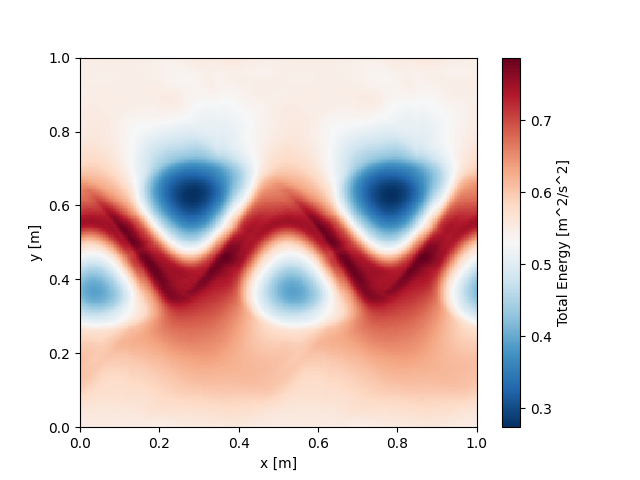
Below is an example that uses the jet initial condition from the shallow water model and demonstrates the three different methods for running the model.
import fridom.shallowwater as sw

# Create the grid and model settings
grid = sw.grid.cartesian.Grid(N=(256,256), L=(1,1), periodic_bounds=(True, True))
mset = sw.ModelSettings(grid=grid, f0=1, csqr=1)
mset.time_stepper.dt = 0.7e-3
mset.setup()

# Create the initial condition
z = sw.initial_conditions.Jet(mset, width=0.1, wavenum=2, waveamp=0.05)

# Create the model and run it
model = sw.Model(mset)
model.z = z  # set the initial condition
model.run(runlen=3)

# Plot the final total energy (kinetic + potential)
model.z.etot.xr.plot(cmap="RdBu_r")
import fridom.shallowwater as sw
# Create the grid and model settings
grid = sw.grid.cartesian.Grid(N=(256,256), L=(1,1), periodic_bounds=(True, True))
mset = sw.ModelSettings(grid=grid, f0=1, csqr=1)
mset.time_stepper.dt = 0.7e-3
mset.setup()
# Create the initial condition
z = sw.initial_conditions.Jet(mset, width=0.1, wavenum=2, waveamp=0.05)
# Create the model and run it
model = sw.Model(mset)
model.z = z # set the initial condition
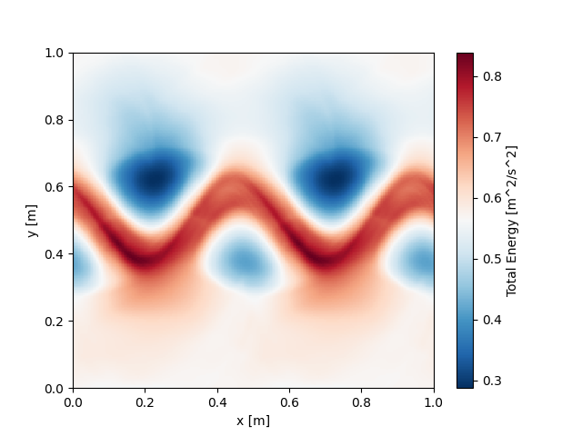
model.run(steps=4000)
# Plot the final total energy (kinetic + potential)
model.z.etot.xr.plot(cmap="RdBu_r")
import fridom.shallowwater as sw
import numpy as np

# Create the grid and model settings
grid = sw.grid.cartesian.Grid(N=(256,256), L=(1,1), periodic_bounds=(True, True))
mset = sw.ModelSettings(grid=grid, f0=1, csqr=1)
mset.time_stepper.dt = 0.7e-3
mset.setup()

# Create the initial condition
z = sw.initial_conditions.Jet(mset, width=0.1, wavenum=2, waveamp=0.05)

# Create the model and run it
model = sw.Model(mset)
model.z = z  # set the initial condition
model.run(start_time=np.datetime64("2020-01-01"),
          end_time=np.datetime64("2020-01-01T00:00:03"))

# Plot the final total energy (kinetic + potential)
model.z.etot.xr.plot(cmap="RdBu_r")
Note
Since 3 seconds do not exactly correspond to 4000 time steps, the resulting plots are not identical.
The choice of method depends on the application. In most cases, the runlen method is recommended. It has the advantage over the steps method that if you change the time step or use an adaptive time-stepping scheme (where time steps vary), the total duration of the model run remains consistent. The method using dates is best suited for simulations of real-world time periods. However, if you are working with idealized setups where the absolute timing is irrelevant, using the runlen method can simplify the process.
Manual Stepping#
You can also manually control the model loop by calling model.step(). However, before starting the loop, you need to invoke the model.start() routine, and after completing the loop, you should call the model.stop() routine. The following example demonstrates this process:
import fridom.shallowwater as sw

# Create the grid and model settings
grid = sw.grid.cartesian.Grid(N=(256,256), L=(1,1), periodic_bounds=(True, True))
mset = sw.ModelSettings(grid=grid, f0=1, csqr=1)
mset.time_stepper.dt = 0.7e-3
mset.setup()

# Create the initial condition
z = sw.initial_conditions.Jet(mset, width=0.1, wavenum=2, waveamp=0.05)

# Create the model
model = sw.Model(mset)
model.z = z  # set the initial condition

# Running the model manually
model.start()
for _ in range(4000):
    model.step()
model.stop()

# Plot the final total energy (kinetic + potential)
model.z.etot.xr.plot(cmap="RdBu_r")
Warning
The progress bar will not work in the above example.
Saving and Loading the Model#
It is possible to save the state of the model and reload it later to continue the simulation. In the example below, we first run the model from the previous examples for 1.5 seconds, then save its state. Afterwards, we load the saved model and continue running it for another 1.5 seconds.
import fridom.shallowwater as sw

# Create the grid and model settings
grid = sw.grid.cartesian.Grid(N=(256,256), L=(1,1), periodic_bounds=(True, True))
mset = sw.ModelSettings(grid=grid, f0=1, csqr=1)
mset.time_stepper.dt = 0.7e-3
mset.setup()

# Create the initial condition
z = sw.initial_conditions.Jet(mset, width=0.1, wavenum=2, waveamp=0.05)

# Create the model
model = sw.Model(mset)
model.z = z  # set the initial condition

# Run the model for 1.5 seconds
model.run(runlen=1.5)

# Save the model
model.save("jet_1.5s")
import fridom.shallowwater as sw

# Create the grid and model settings
grid = sw.grid.cartesian.Grid(N=(256,256), L=(1,1), periodic_bounds=(True, True))
mset = sw.ModelSettings(grid=grid, f0=1, csqr=1)
mset.time_stepper.dt = 0.7e-3
mset.setup()

# Create the model
model = sw.Model(mset)

# Load the model
model.load("jet_1.5s")

# Run the model for another 1.5 seconds
model.run(runlen=1.5)

# Plot the final total energy (kinetic + potential)
model.z.etot.xr.plot(cmap="RdBu_r")
Summary#
In this tutorial, we covered the basics of running a model using the FRIDOM framework. We started by explaining how to initialize a grid and configure model settings before creating the model itself. We then explored different methods to run the model: specifying the duration using runlen, the number of steps with steps, or defining a time range with date. Each approach has its advantages, with runlen often being the most practical for most applications, especially when working with varying time steps.
Additionally, we demonstrated how to manually control the model loop using model.step(), which allows for more granular control over each time step. Finally, we showed how to save and load the model state to pause and resume simulations, which is useful for running longer experiments in multiple stages. Together, these techniques provide a flexible and powerful way to perform and analyze simulations with FRIDOM.
In the next tutorial, we will introduce the concepts of FRIDOM’s module. These will become relevant if you want to write model output to netCDF files, if you want to create animations, or if you want to modify the model’s behavior.