Modules Part 1: Understanding Modules

A FRIDOM module is a component of the model that includes an update method. The update method takes the module state, performs an operation, and returns the updated state. Modules can compute tendency terms (e.g., the tendency due to Coriolis force) or serve diagnostic purposes (e.g., computing the global mean surface temperature every 20 timesteps and writing it to a file). They allow you to modify and extend the model without altering its core.

In this tutorial, you will learn:

• What the ModelState object is (the object passed to the update method),

• How FRIDOM’s module structure works (e.g., when specific modules are called),

• How to add, disable, and enable modules in the model.

ModelState

The ModelState contains all relevant information about the model’s current state, including the following attributes:

Component	Type	Description
z	VectorField	Prognostic state vector
dz	VectorField	Tendency of the prognostic state vector
z_diag	VectorField	State vector with diagnostic variables
clock	Clock	Information about the model time

You typically don’t need to create a ModelState manually; it is initialized automatically when the model is set up. Instead, you interact with the existing ModelState object. The following example demonstrates accessing the ModelState object and its attributes.

Accessing the ModelState object

import fridom.shallowwater as sw

# Create the grid and model settings as usual
grid = sw.grid.cartesian.Grid(N=(256, 256), L=(1, 1), periodic_bounds=(True, True))
mset = sw.ModelSettings(grid=grid)
mset.setup()

# Create the model
model = sw.Model(mset)

# Access the ModelState object
mz = model.model_state

# From here, you can access the above mentioned attributes,
# for example the clock or the state variables
print(mz.clock)
print(mz.z)

Output

Clock(
  start_time = 0,
  passed_time = 0,
  current_time = 0)
State(
  u=u - velocity  [m/s],
  v=v - velocity  [m/s],
  p=pressure  [m²/s²],
)

Tip

The model state is abbreviated as mz to keep the code concise. Whenever you see mz, it refers to the model state.

The Standard Modules in FRIDOM Models

FRIDOM models follow a specific module structure, which determines the sequence of computations for each time step. The standard modules included in all FRIDOM models are:

Modulename	Description
tendencies	Compute time tendency terms
diagnostics	Perform diagnostics (e.g. output to file)
time_stepper	Perform the time stepping
nan_checker	Check state vector for NaNs
progress_bar	Display a progress bar
restart_module	Perform restart operations on computing clusters

The tendencies and diagnostics modules are particularly important. These modules act as containers for sub-modules, providing an interface for adding custom modules (e.g., for turbulence closures or animation generation). Adding, enabling, and disabling modules is covered in the final section of this tutorial. First, let’s see how to access these modules.

You can access modules via either the ModelSettings class or the Model class. Both provide access to the same objects. The following example demonstrates how to access the tendencies module from both the ModelSettings and Model classes.

Inspect Tendency

import fridom.shallowwater as sw

# Create the grid and model settings and model as usual
grid = sw.grid.cartesian.Grid(N=(256, 256), L=(1, 1), periodic_bounds=(True, True))
mset = sw.ModelSettings(grid=grid)
mset.setup()
model = sw.Model(mset)

# Access the tendency module from the model and from the model settings
tendencies = model.tendencies
# Let's see what the tendencies module looks like
print(tendencies)

Output

Module Container
## Reset Tendency
## Linear Tendency
## Sadourny Advection
  - Required Halo: 2

Accessing a module

import fridom.shallowwater as sw

# Create the grid and model settings and model as usual
grid = sw.grid.cartesian.Grid(N=(256, 256), L=(1, 1), periodic_bounds=(True, True))
mset = sw.ModelSettings(grid=grid)
mset.setup()
model = sw.Model(mset)

print("Model and model settings point to the same tendencies module:")
print(id(model.tendencies) == id(mset.tendencies))

Output

Model and model settings point to the same tendencies module:
True

From the output of the “Inspect Tendency” example, you can see that the tendencies module is a ModuleContainer that contains three modules. These modules are called in the order they appear in the list. In this case, the Reset Tendency module is called first, setting the tendency variables to zero. Next, the Linear Tendency module is called, which computes the linear tendency terms. Finally, the Sadourny Advection module is called, which computes the nonlinear advection terms.

Time Step Sequence

We now have enough information to understand the time step sequence of FRIDOM models. Let’s look at the source code of the Model class, which controls the time step sequence:

The time step method of the Model class

def step(self) -> None:
    """Update the model state by one time step."""
    # synchronize the state vector (ghost points)
    with self.timer["sync"]:
        self.z.sync()

    # perform the time step
    self.model_state = self.time_stepper.update(mz=self.model_state)

    # check if there are any nans in the state variable
    self.model_state = self.nan_checker.update(self.model_state)

    # make diagnostics
    self.model_state = self.diagnostics.update(mz=self.model_state)

    # Update the progress bar
    self.progress_bar.update(self.model_state)

    # check if the model should restart
    if self.restart_module.should_restart(self.model_state):
        self.restart_module.restart(self)

Note

In the example above, self refers to the object of the Model class.

Let’s go through the code step by step:

1. The sync method synchronizes the ghost points between processors.

2. The update method of the time_stepper module is called, stepping the state variables forward in time.

3. The update method of the nan_checker module is called to check for NaNs in the state vector. If NaNs are found, the model will stop.

4. Diagnostics, as for example writing to a file, are performed using the update method of the diagnostics module.

5. The progress bar is updated.

6. The restart_module checks if the model should restart (only relevant for computing clusters).

You may wonder, where the tendency terms are computed, since the tendencies module is not called in the time step method. The tendencies module is called in the update method of the time_stepper module. This is an intended design choice to allow for flexibility in the implementation of different time steppers. For example, a Runge-Kutta time stepper may call the tendencies module multiple times to compute intermediate steps while the Adam Bashforth time stepper only calls it once. If you want to learn more about the time steppers in FRIDOM, you may want to have a look at this tutorial.

Manipulating Modules

When working with FRIDOM models, it is almost always necessary to modify the standard modules. Let’s start with the most basic operations: disabling and enabling modules. This is done using the disable() and enable() methods. For example the followin code demonstrates how to disable the advection module:

Disabling Advection Module

import fridom.shallowwater as sw

# Create the grid and model settings
grid = sw.grid.cartesian.Grid(N=(256,256), L=(1,1), periodic_bounds=(True, True))
mset = sw.ModelSettings(grid=grid, f0=1, csqr=1)
mset.time_stepper.dt = 0.7e-3
mset.tendencies.advection.disable()
mset.setup()

# Create the initial condition
z = sw.initial_conditions.Jet(mset, width=0.1, wavenum=2, waveamp=0.05)

# Create the model and run it
model = sw.Model(mset)
model.z = z  # set the initial condition
model.run(runlen=3)

# Plot the final total energy (kinetic + potential)
model.z.etot.xr.plot(cmap="RdBu_r")

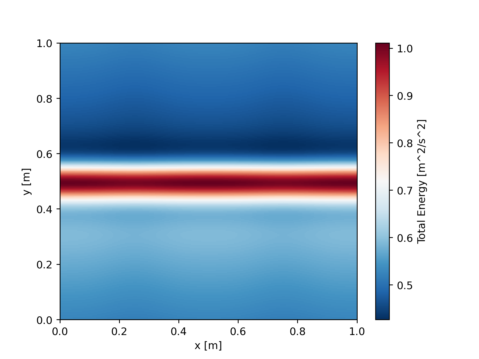
Since the jet does not get instable without the nonlinear advection terms, the result is not very interesting. However, that is not the point of this example. Instead, it demonstrates how to disable a module. You can of course disable any other module in the same way. For example, you could try to disable the progress bar in the above example.

Adding Custom Modules

Finally, let’s add a custom module to the model. To do this, you need to create a module object and add it to the module container of the model settings. Don’t forget to call the setup() method of the model settings object after adding all modules. In the following example, we add a friction module to the shallow water model:

with friction

import fridom.shallowwater as sw

# Create the grid and model settings
grid = sw.grid.cartesian.Grid(N=(256,256), L=(1,1), periodic_bounds=(True, True))
mset = sw.ModelSettings(grid=grid, f0=1, csqr=1)
mset.time_stepper.dt = 0.7e-3

# we create a friction module, and add it to the tendency container
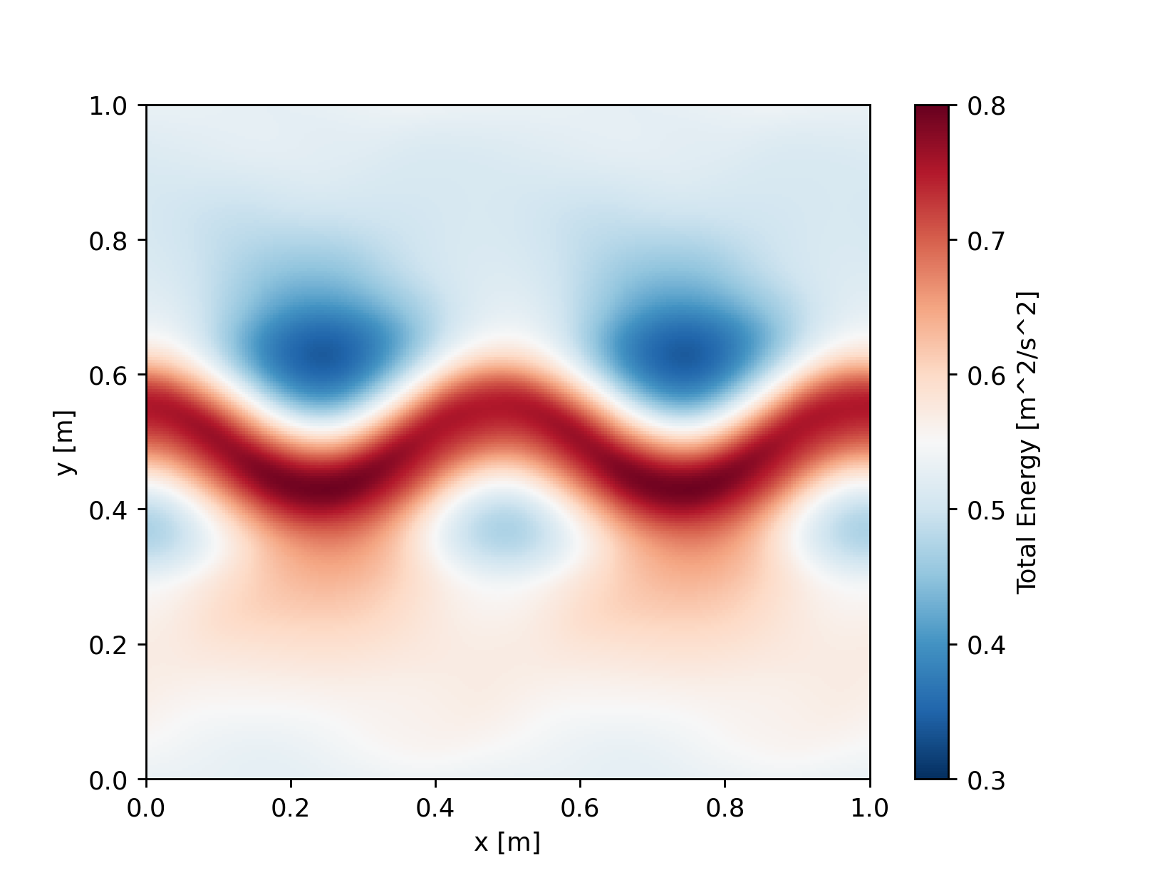
friction = sw.modules.closures.HarmonicFriction(ah=3e-4)
mset.tendencies.add_module(friction)

mset.setup()

# Create the initial condition
z = sw.initial_conditions.Jet(mset, width=0.1, wavenum=2, waveamp=0.05)

# Create the model and run it
model = sw.Model(mset)
model.z = z  # set the initial condition
model.run(runlen=3)

# Plot the final total energy (kinetic + potential)
model.z.etot.xr.plot(cmap="RdBu_r", vmin=0.3, vmax=0.8)

without friction

import fridom.shallowwater as sw

# Create the grid and model settings
grid = sw.grid.cartesian.Grid(N=(256,256), L=(1,1), periodic_bounds=(True, True))
mset = sw.ModelSettings(grid=grid, f0=1, csqr=1)
mset.time_stepper.dt = 0.7e-3

mset.setup()

# Create the initial condition
z = sw.initial_conditions.Jet(mset, width=0.1, wavenum=2, waveamp=0.05)

# Create the model and run it
model = sw.Model(mset)
model.z = z  # set the initial condition
model.run(runlen=3)

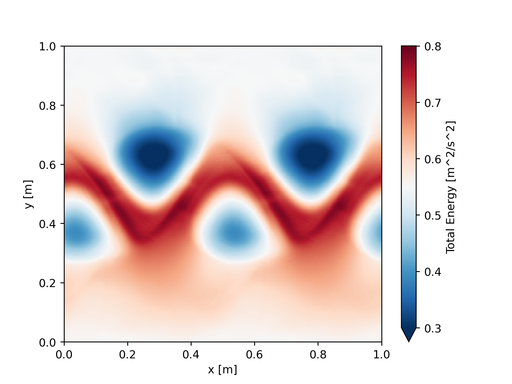
# Plot the final total energy (kinetic + potential)
model.z.etot.xr.plot(cmap="RdBu_r", vmin=0.3, vmax=0.8)

Similar to adding modules to the tendency container, you can also add modules to the diagnostics container. We will do this in the next tutorial, where we add a netCDF output writer to the model.