EquatorialWave

class fridom.shallowwater.initial_conditions.equatorial_wave.EquatorialWave(mset: ModelSettings, longitudinal_mode: int, equatorial_mode: int, wave_mode: int, phase: float = 0)

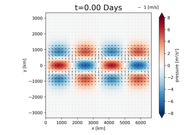
Bases: State

Equatorial wave on the beta-plane approximation.

Parameters

msetModelSettings

Model settings.

longitudinal_modeint

Longitudinal mode of the wave (how many wavelengths in the x-direction).

equatorial_modeint

Equatorial mode of the wave (Hermite polynomial order).

wave_modeint

Mode of the wave:

0 for the wave mode with negative frequency 1 for the rossby mode (smallest absolute frequency) 2 for the wave mode with positive frequency

phasefloat, optional

Phase of the wave.

Description

The equatorial wave solutions follow from solving the eigenvalue problem of the linearized shallow water equations on the equatorial beta-plane \(f = \beta y\). The frequencies of the m-th eigenmode can be obtained by solving

\[\omega_m \left( \omega_m^2 - c^2 \left( k^2 + (2m + 1) \frac{\beta}{c} \right) \right) = k \beta c^2\]

for \(\omega_m\).

The initial condition is then given by

\[\begin{split}\mathbf z = \begin{pmatrix} u_m \\ v_m \\ p_m \end{pmatrix} e^{- \frac{1}{2}\tilde{y}^2} e^{i(kx + \phi)} \quad \text{with} \quad \tilde{y} = \frac{y}{R_e} \quad \text{and} \quad R_e^2 = \frac{c}{\beta}\end{split}\]

with

\[\begin{split}\begin{align} u_m &= \frac{i c}{2 R_e} \left( \frac{H_{m+1}(\tilde{y})}{\omega_m - c k} + \frac{2 m H_{m-1}(\tilde{y})}{\omega_m + c k} \right) \\ v_m &= H_m(\tilde{y}) \\ p_m &= \frac{i c^2}{2 R_e} \left( \frac{H_{m+1}(\tilde{y})}{\omega_m - c k} - \frac{2 m H_{m-1}(\tilde{y})}{\omega_m + c k} \right) \end{align}\end{split}\]

where \(H_m\) is the m-th Hermite polynomial, given by the recursive relation

\[H_m(x) = 2x H_{m-1}(x) - 2(m-1) H_{m-2}(x)\]

with \(H_{-1}(x) = 0\) and \(H_0(x) = 1\).

__init__(mset: ModelSettings, longitudinal_mode: int, equatorial_mode: int, wave_mode: int, phase: float = 0) → None

Methods

__init__(mset, longitudinal_mode, ...[, phase])
abs()	Map the field by taking the absolute value (\(|f|\)).
apply_elementwise(vector_field, op)	Apply an operation elementwise to the vector field.
apply_water_mask()	Apply a water mask to the field.
conj()	Compute the complex conjugate.
cumulative_integral(axis[, direction])	Compute the cumulative integral along an axis.
diff(axis[, order])	Compute the partial derivative along an axis.
div()	Compute the divergence.
dot(other)	Compute the dot product with another field.
extend(topo)	Extend the field in the specified directions.
fft([padding])	Perform a Fast Fourier Transform (FFT) on the field.
from_netcdf(mset, path)	Create a field from a NetCDF file.
from_xarray(mset, ds)	Create a field from an xarray object.
grad([axes])	Compute the gradient.
has_nan()	Check if the field contains NaN values.
ifft([padding])	Perform an Inverse Fast Fourier Transform (IFFT) on the field.
integrate([axes])	Global integral of the Field in specified axes.
laplacian([axes])	Compute the Laplacian.
max([axes])	Maximum value of the Field over the whole domain.
mean([axes])	Global mean of the Field in specified axes.
min([axes])	Minimum value of the Field over the whole domain.
norm_l2()	Calculate the L2 norm of the field.
norm_of_diff(other)	Norm of difference between two vector fields.
project(p_vec, q_vec)	Project a Vector Field onto a (spectral) vector.
set_random([seed])	Set the field to random values.
sum([axes])	Sum of the Field over the whole domain in the specified axes.
sync()	Synchronize the field across all MPI ranks and apply boundary conditions.
to_netcdf(path)	Save the field to a NetCDF file.

Attributes

cfl	The CFL number.
ekin	Vertically integrated kinetic energy.
epot	Vertically integrated kinetic energy.
etot	The total energy.
field_list	The list of scalar fields.
fields	The dictionary of scalar fields.
grid	The grid object.
info	Dictionary with information about the field.
is_constant	Flag indicating whether the field is constant.
is_spectral	Flag indicating whether the field is in spectral space.
local_rossby_number	Local Rossby number.
mset	The model settings.
p	Pressure \(p\).
pot_vort	Scaled potential vorticity field.
rel_vort	Relative vorticity.
spectral_ekin	Spectral kinetic energy density.
tracers	The tracer fields.
u	Velocity in the x-direction.
v	Velocity in the y-direction.
vector_dim	The vector dimension.
velocity	Velocity vector.
xr	The xarray representation of the field.
xrs	Convert a slice of the field to an xarray object.

Examples using fridom.shallowwater.initial_conditions.EquatorialWave

Equatorial Waves.

Equatorial Waves.