BarotropicJet

class fridom.nonhydro.initial_conditions.barotropic_jet.BarotropicJet(mset: ModelSettings, wavenum=5, waveamp=0.1, jet_width=0.04, geo_proj=True)

Bases: State

Barotropic instable jet setup with 2 zonal jets

Description

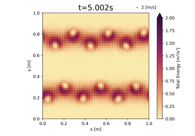
A Barotropic instable jet setup with 2 zonal jets and a perturbation on top of it. The jet is given by:

\[u = 2.5 \left( \exp\left(-\left(\frac{y - 0.75 L_y}{\sigma L_y \pi}\right)^2\right) - \exp\left(-\left(\frac{y - 0.25 L_y}{\sigma L_y \pi}\right)^2\right) \right)\]

where \(L_y\) is the domain length in the y-direction, and \(\sigma\) is the width of the jet. The perturbation is given by:

\[v = A \sin \left( \frac{2 \pi}{L_x} k_p x \right)\]

where \(A\) is the amplitude of the perturbation and \(k_p\) is the wavenumber of the perturbation. When geo_proj is set to True, the initial condition is projected to the geostrophic subspace using the geostrophic eigenvectors.

Parameters

msetModelSettings

The model settings.

wavenumint

The wavenumber of the perturbation.

waveampfloat

The amplitude of the perturbation.

jet_widthfloat

The width of the jet.

geo_projbool

Whether to project the initial condition to the geostrophic subspace.

__init__(mset: ModelSettings, wavenum=5, waveamp=0.1, jet_width=0.04, geo_proj=True)

Methods

__init__(mset[, wavenum, waveamp, ...])
abs()	Map the field by taking the absolute value (\(|f|\)).
apply_elementwise(vector_field, op)	Apply an operation elementwise to the vector field.
apply_water_mask()	Apply a water mask to the field.
conj()	Compute the complex conjugate.
cumulative_integral(axis[, direction])	Compute the cumulative integral along an axis.
diff(axis[, order])	Compute the partial derivative along an axis.
div()	Compute the divergence.
dot(other)	Compute the dot product with another field.
extend(topo)	Extend the field in the specified directions.
fft([padding])	Perform a Fast Fourier Transform (FFT) on the field.
from_netcdf(mset, path)	Create a field from a NetCDF file.
from_xarray(mset, ds)	Create a field from an xarray object.
grad([axes])	Compute the gradient.
has_nan()	Check if the field contains NaN values.
ifft([padding])	Perform an Inverse Fast Fourier Transform (IFFT) on the field.
integrate([axes])	Global integral of the Field in specified axes.
laplacian([axes])	Compute the Laplacian.
max([axes])	Maximum value of the Field over the whole domain.
mean([axes])	Global mean of the Field in specified axes.
min([axes])	Minimum value of the Field over the whole domain.
norm_l2()	Calculate the L2 norm of the field.
norm_of_diff(other)	Norm of difference between two vector fields.
project(p_vec, q_vec)	Project a Vector Field onto a (spectral) vector.
set_random([seed])	Set the field to random values.
sum([axes])	Sum of the Field over the whole domain in the specified axes.
sync()	Synchronize the field across all MPI ranks and apply boundary conditions.
to_netcdf(path)	Save the field to a NetCDF file.

Attributes

b	Buoyancy.
cfl	The CFL number.
ekin	The kinetic energy.
epot	The potential energy.
etot	The total energy.
field_list	The list of scalar fields.
fields	The dictionary of scalar fields.
grid	The grid object.
info	Dictionary with information about the field.
is_constant	Flag indicating whether the field is constant.
is_spectral	Flag indicating whether the field is in spectral space.
linear_pot_vort	Linearized potential vorticity.
local_rossby_number	Local Rossby number.
mset	The model settings.
pot_vort	Scaled potential vorticity field.
rel_vort	The relative vorticity.
rel_vort_x	X-component of the relative vorticity.
rel_vort_y	Y-component of the relative vorticity.
rel_vort_z	Z-component of the relative vorticity (horizontal vorticity).
tracers	The tracer fields.
u	Velocity in the x-direction.
v	Velocity in the y-direction.
vector_dim	The vector dimension.
velocity	The velocity vector field.
w	Velocity in the z-direction.
xr	The xarray representation of the field.
xrs	Convert a slice of the field to an xarray object.

Examples using fridom.nonhydro.initial_conditions.BarotropicJet

Barotropic Jet

Barotropic Jet